Equilibrium Values and their Stability for First-Order Non-Linear DDS

In Section 6.5 we have derived a formula to determine the equilibrium value for a first-order
linear DDS and also a criterion to determine the stability of the equilibrium value. Unfortunately,
we will not be able to derive such a general formula for a first-order non-linear DDS. However,
we can use the same approach for finding the equilibrium as we did in case of a linear DDS.
Recall that for a system in equilibrium, the new output value is equal to the old output value, i.e.,
no change occurs. Thus, if the system is given in the form

x(n +1) = f (x(n))

then this requirement for the equilibrium becomes

x(n) = x(n +1) = f (x(n)).

If we again denote the equilibrium value by x, we need to solve the following equation:

x = f (x) .

A value that solves this equation is called a fixed point of the function f. We summarize this in the
following theorem.

Here is an example:
We want to find the equilibrium value(s) for the DDS given by x(n +1) = 5x(n)² . The model
function f (= right hand side of the iterative model equation) is given by f (x(n)) = 5x(n)² . To
find the equilibrium, we have to solve the following equation:

x = f (x) or x = 5x² .

To find the solution(s), we can use either the palette function SolveIt or analytical methods
(depending on your mathematics background). Here is how to do this with SolveIt. Recall that
SolveIt has as entries the left hand side and the right hand side of the equation, as well as the
variable to be solved for.



The resulting output is



This indicates that both x = 0 and are equilibrium values. We can verify this by substituting
these values into the original equation.

To solve the above equation analytically, we use methods to solve quadratic equations. We start
by moving all terms to one side of the equation. The next step is to look whether factoring is
possible. If not, apply the quadratic formula (see appendix, A4).



If a product is zero, then either one or both of the factors has to be zero. This implies that either



Again, both x = 0 and are the equilibrium values.

Graphically, we can find fixed points of the function f by drawing the graph of the function
together with the line y = x , the 45° line. The x-values of the points at which the graph intersects
the 45° line are the fixed points or equilibrium values. Why is that the case? Remember that in this
graph, the input value is given by x(n) (on the horizontal axis), and the output value is given by
f (x(n)) (on the vertical axis). At the 45° line, the two values are identical, hence
x(n) = f (x(n)) = x(n + 1). Thus, the system is in equilibrium for this input value. We will illustrate
this method for the example above, x(n +1) = 5x(n)² .

From the graph, we identify the points of intersection, (0,0) and (0.2, 0.2), respectively. Their
input values, namely 0 and 0.2 = 1/5, are the two equilibrium values.

We now turn to determining the stability of the equilibrium values for a non-linear DDS. The
criterion is still the same:

• If the initial value is slightly above or below the equilibrium value and the sequence of system
values converges (= gets close) to that equilibrium value, then the equilibrium is stable.
• If the initial value is slightly above or below the equilibrium value and the sequence of system
values diverges away from that equilibrium value, then the equilibrium is unstable.
• If the sequences of system values for initial value slightly above or below the equilibrium value
exhibit both converging and diverging behavior, then the equilibrium is semi-stable. In all
other cases, the equilibrium is neutral.

To determine stability, we can look at a table of values or a Cobb-web diagram. Let's start with
the table. In the previous example, x(n +1) = 5x(n)² , we found that the equilibrium values are
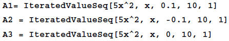
x = 0 and x = 0.2. We first check the equilibrium value x = 0 for stability. We can create a
sequence of values using the palette function IteratedValueSeq. As starting values we can use
0.1 and -0.1. (Be careful not to chose a value that is bigger than the second equilibrium value
0.2.) In order to graph the sequences later, we give each one a name and also create a sequence
starting at the equilibrium value.

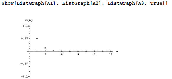
The table below summarizes the results (to six decimal places).

Since the values for x(n) approach zero, no matter whether we start slightly above or slightly
below the equilibrium value, x = 0 is a stable equilibrium. We can visualize this behavior by using
the built-in Mathematica function Show. Note that the values for the equilibrium sequence are
connected by a line because we used the (optional) value of True in the last ListGraph
command.

Now we will look at how a Cobb-web diagram or (Cobb-web graph) is constructed. We start by
graphing the model function f together with the 45° line (where x(n +1) = x(n)). The horizontal
axis displays the values for x(n) (=input values) and the vertical axis displays the values
for x(n +1) (= output values). We will use horizontal and vertical lines to read off the next output
value and to translate this value from the vertical axis to the horizontal axis (so it becomes the
next input value). First, we draw a vertical line through the initial value x(0) until this line
intersects with the graph of the model function f . The corresponding output value can be read
off by drawing a horizontal line from the intersection point to the vertical axis. This gives the
value of x(1) . Below is an illustration of the procedure for the iterative model equation
x(n +1) = 5x(n)² with initial value x(0) = 0.1. . In this case, x(1) = 0.05.